Logistic and Softmax Regression

In this post, I try to discuss how we could come up with the logistic and softmax regression for classification. I also implement the algorithms for image classification with CIFAR-10 dataset by Python (numpy). The first one) is binary classification using logistic regression, the second one is multi-classification using logistic regression with one-vs-all trick and the last one) is mutli-classification using softmax regression.

1. Problem setting

Classification problem is to classify different objects into different categories. It is like regression problem, except that the predictor y just has a small number of discrete values. For simplicity, we just focus on binary classification that y can take two values 1 or 0 (indicating two classes).

2. Basic idea

We could plot the data on a 2-D plane and try to figure out whether there is any structure of the data (see following figure).

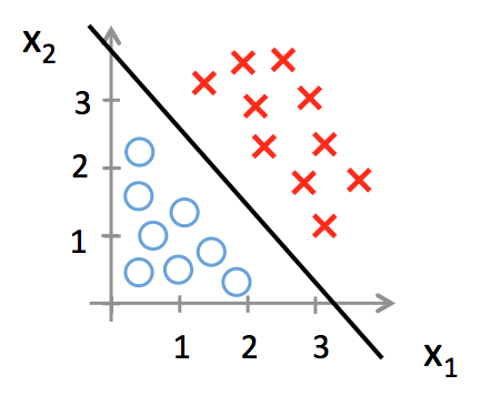
From the particular example above, it is not hard to figure out we could find a line to separate the two classes. Specifically we divide the 2-D plane into 2 parts according to a line, and then we can predict new sample by observing which part it belongs to. Mathematically if \(z = w_0 + w_1x_1 + w_2x_2\) >= 0, then y = 1; if \(z = w_0 + w_1x_1 + w_2x_2\) < 0, then y = 0. We can regard the linear function \(w^Tx\) as a mapping from raw sample data (\(x_1, x_2\)) to classes scores. Intuitively we wish that the “correct” class has a score that is higher than the scores of “incorrect” classes.

3. How to find the best line

The hypothesis is a linear model \(w_0 + w_1x_1 + w_2x_2 = W^TX\), the threshold is z = 0. The score value of z depends on the distance between the point and the target line, and the absolute value of z could be very large or small. We could normalize the distances for convenience, however, we had better not use linear normalization such as x / (max(x) - min(x)) and x / (std(x)), because the distinction between the two classes is more obvious when the absolution value of z is larger. Sigmoid or logistic function is well-known to be used here, following is the function and plot of sigmoid function.

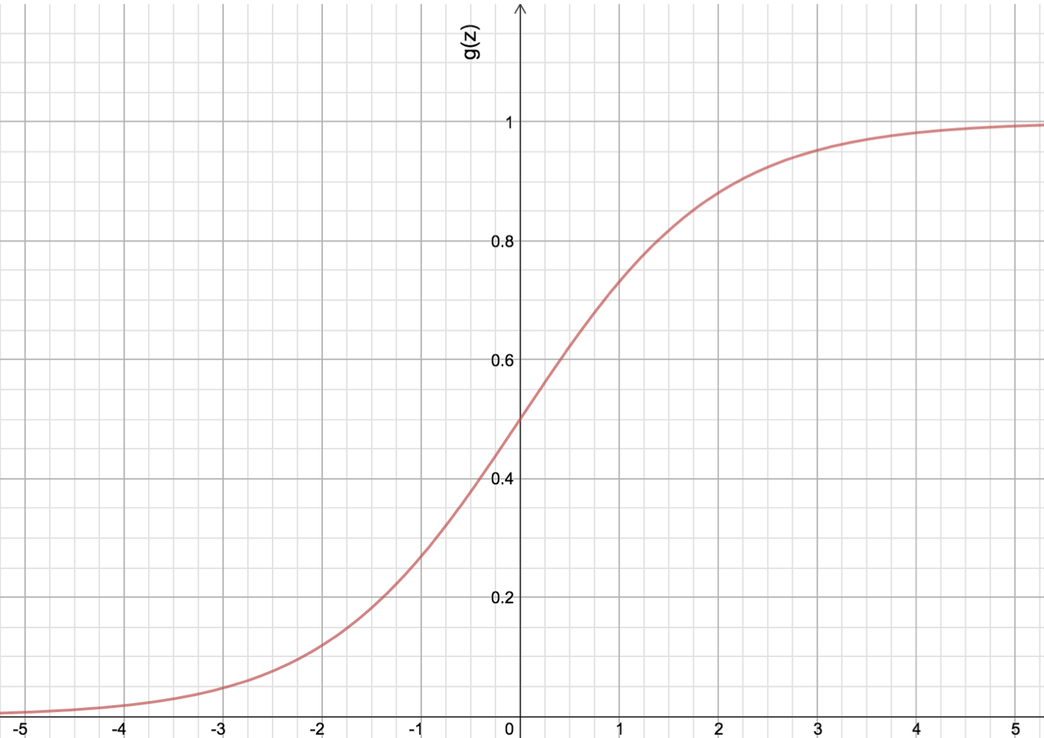
The new model for classification is:

\(h(x) = \frac{1}{1 + e^{-w^Tx}}\) We can see from the figure above that when z 0, g(z) 0.5 and when the absolute vaule of v is very large the g(z) is more close to 1. By feeding the score to sigmoid function, not only the scores can be normalized from 0 to 1, which can make it much easier to find the loss function, but also the result can be interpreted from probabilistic aspect.

4. Figure out the loss function

we need to find a way to measure the agreement between the predicted scores and the ground truth value.

Naive idea

We could use least square loss after normalizing the training data, the result is as following: \(L_0 = \frac{1}{m} \sum_{i=1}^m(h(x^{(i)}) - y^{(i)})^2 = \frac{1}{m} \sum_{i=1}^m(\frac{1}{1 + e^{-w^Tx^{(i)}}} - y^{(i)})^2\), where \(x^{(i)}\) is a vector for all features \(x_j^{(i)}\) (j=0,1, … , n) for single sample i, and \(y^{(i)}\) is the target value for this example. However this loss function is not a convex function because of sigmoid function used here, which will make it very difficult to find the w to opimize the loss.

Can we do better?

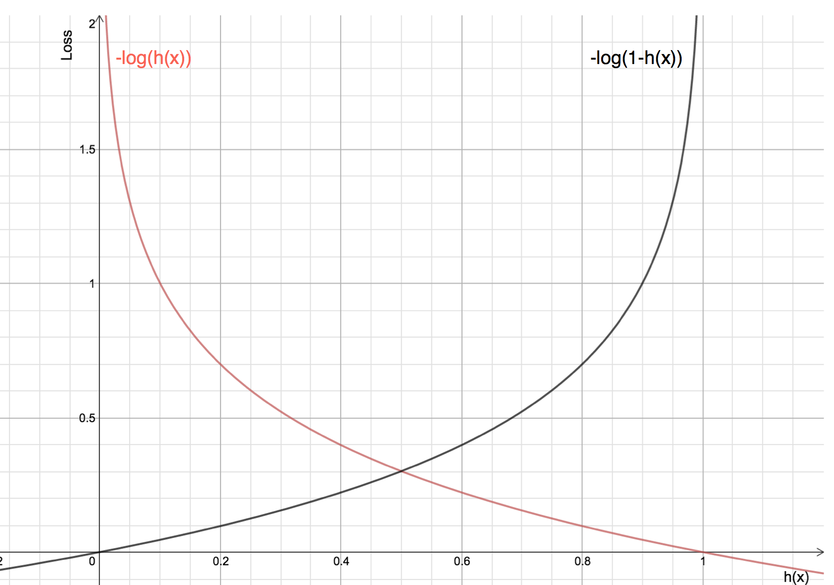
Because of this is a binary classification problems, we can compute the loss for the two classes respectively. When target y = 1, the loss had better be very large when \(h(x) = \frac{1}{1 + e^{-w^Tx}}\) is close to zero, and the loss should be very small when h(x) is close to one; in the same way, when target y = 0, the loss had better be very small when h(x) is close to zero, and the loss should be very large when h(x) is close to one. In fact, we can find this kind of function:

So the total loss: \(L(w) = - \frac{1}{m} \sum_{i = 1}^m [y^{(i)}logh(x^{(i)}) + (1 - y^{(i)}) log(1-h(x^{(i)}))]\)

\(x^{(i)}\) is a vector for all \(x_j\) (j=0,1, … , n), and \(y^{(i)}\) is the target value for this example.

The plots of loss function are shown below, and they meet the desirable properties discribed above.

5 Find the best w to minimize the loss

Like linear regression we can use gradient descent algorithm to optimize w step by step. Compute the gradient for just one sample:

So the gradients are as following when considering all the samples:

Then we can use batch decent algorithm or stochastic decent algorithm to optimize w, i.e, \(w := w + \alpha \frac{\partial}{\partial w_j} L(w)\)

We can see that the gradient or partial derivative is the same as gradient of linear regression except for the h(x). We can get a better understanding of this when interpreting the loss function from probabilistic aspect.

6. Probabilistic interpretation

Let us regard the value of h(x) as the probability:

So the likelihood is:

And the log likelihood:

This equation is the same as the the loss function when picking minus, so minimize the loss can be interpreted as maximize the likelihood of the y when given x p(y|x). What’s more, the value of h(x) can be interpreted as the probability of the sample to be classified to y = 1. I think this is why most people prefer sigmoid function for normalization, theoretically we can choose other functions that smoothly increase from 0 to 1.

After we optimize the w, we get a line in 2-D space and the line is usually called decision boundary (h(x) = 0.5). We can also generalize to binary classification on n-D space, and the corresponding decision boundary is a (n-1) Dimension hyperplane (subspace) in n-D space.

7. Multiclass classification – One vs all

We need to generalize to the multiple class case, that’s to say, the value of y is not binary any more, instead y can equal to 0, 1, 2, …, k.

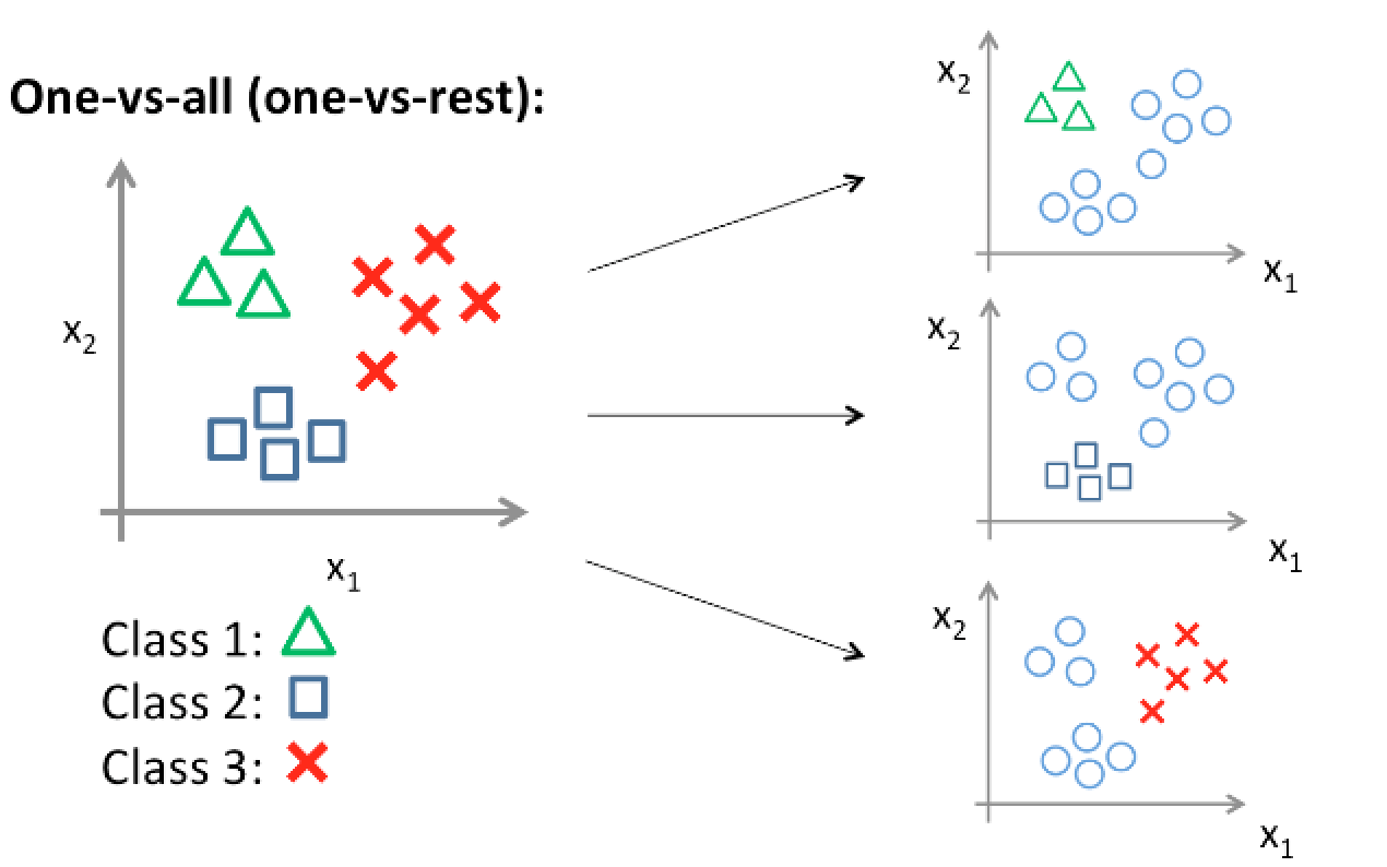
Basic idea – Transfer multi-class classification into binary classification problem

We need change multiple classes into two classes, and the idea is to construct several logistic classifier for each class. We set the value of y (label) of one class to 1, and 0 for other classes. Thus, if we have K classes, we build K logistic classifiers and use it for prediction. There is a potential problem that one sample might be classified to several classes or non-class. The solution is to compare all the values of h(x) and classify the sample to the class with the highest value of h(x). The idea is shown in following figure (From Andrew’s notes).

8. Can we do better? – Softmax

In logistic regression classifier, we use linear function to map raw data (a sample) into a score z, which is feeded into logistic function for normalization, and then we interprete the results from logistic function as the probability of the “correct” class (y = 1). We just need a mapping function here because of just two classes (just need to decide whether one sample belongs to one class or not). For multiple classes problems (K categories), it is possible to establish a mapping function for each class. As above we can simply use a linear mapping for all classes (K mapping function):

Where \(x^{(i)}\) is a vector for all features \(x_j^{(i)}\) (j=0,1, … , n) for single sample i, and \(x^{(i)}\) is a single column vector of shape \([D, 1]\). W is a matrix of shape \([K, D]\) called weights, K is the number of categories, and b is a vector of \([K, 1]\) called bias vector. It is a little cumbersome to keep track of two sets of parameters (W and b), in factor we can combine the two into a single matrix. Specifically we can extend the feature vector \(x^{(i)}\) with an addition bias dimension holding constant 1, while extending W matrix with a new column (at the first or last column). Thus we get score mapping function:

Where W is a matrix of shape \([K, D+1]\), \(x^{(i)}\) is vector of shape \([D+1, 1]\), and \(f(x^{(i)}, W)\) is a vector of shape \([K, 1]\) indicating the different scores of every class for the \(i^{th}\) sample.

Find the loss function

Similar to logistic regression classifier, we need to normalize the scores from 0 to 1. However we should not use a linear normalization as discussed in the logistic regression because the bigger the score of one class is, the more chance the sample belongs to this category. What’s more, the chance is similar high when the scores are very large (see the plot of logistic function above). Similar to logistic function, people use exponential function (non-linear) to preprocess the scores and then compute the percentage of each score in the sum of all the scores. What’s more, the percentages can be interpreted as the probability of each class for one sample. Here is formula for the \(i^{th}\) sample:

Here is the plot of h(x) for two classes in 3D space, you can rotate the graph by clicking the arrows to get a better understanding the shape of the h(x). Where \(x^{(i)}\) is vector of all features of sample i, \(w_j\) is the weights for the \(j^{th}\) class, and \(y_j\) is the correct class for the \(i^{th}\) sample.

So why exponential function? In my opinion, it is natually to come up with.

• It is a very simple and widely used non-linear function
• This function is strictly increasing
• This function is a convex function and its derivative is strictly increasing. That’s to say, when the score is large, then make it even more larger.

The lesson is that we should put exponential function in our toolbox for non-linear problems

After normalizing the scores, we can use the same concept to define the loss function, which should make the loss small when the normalized score of h(x) is large, and penlize more when h(x) is small. Thus, we can use \(-log(h(x))\) to compute the loss, and the loss for one sample is as following:

Total loss for all sample is:

Calculate the gradient (one sample)

So the gradient with respect to \(w_{y_j}\) (\(y_j\) is the correct class): \(\nabla_{w_{y_j}} = -x^{(i)} + \frac{e^{w_j^Tx^{(i)}}} {\sum_{j = 1}^k e^{w_j^Tx^{(i)}}} x^{(i)}\)

The gradient with respect to \(w_j\): \(\nabla_{w_j} = \frac{e^{w_j^Tx^{(i)}}} {\sum_{j = 1}^k e^{w_j^Tx^{(i)}}} x^{(i)}\)

Is there any problem with the loss function

When writing code to implement the softmax function in practice, we should first compute the intermediate terms \(e^{f_j}\) to make the scores bigger and use a logarithm function to make the score smaller. However, the value of \(e^{f_j}\) may be very large due to the exponentials and dividing large numbers could be numerically unstable, so we should make \(e^{f_j}\) smaller before division. Here is the trick by multiply the numerator and denominator by a constant C:

Because we have the flexibility to choose any number of C, we can choose C to make \(e^{f_j^{(i)}} + logC\) small. A common choice for C is to set \(logC = -max_jf_j^{(i)}\). This trick makes the highest value of \(f_j^{(i)} + logC\) to be zero and less than 0 for others. So the values of \(e^{f_j^{(i)}} + logC\) are restricted from 0 to 1, which should be more appropriate for division.

Probabilistic interpretation

We can interpret \(h(x) = P(y^{(i)}) = \frac{e^{w_{y_j}^Tx^{(i)}}} {\sum_{j = 1}^k e^{w_j^Tx^{(i)}}}\) as the normalized probability of assigned to the correct label \(y^{(i)}\) given sample x^{(i)} and parameters W. Firstly the score \(f(x^{(i)}, W) = Wx^{(i)}\) can be interpreted as the unnormalized log probabilities. Then exponentiating the scores with on-linear function \(e^x\) gives the unnormalized probabilities (may call frequency). Last using division for normalization to make the probabilities sum to one. Like logistic regression, the minimize the negative log likelihood of the correct class can also be interpreted as performing Maximum Likelihood Estimation. The loss function can be also deduced from probabilistic theory like logistic regression, in fact linear regression, logistic regression and softmax regression all belong to Generalized Linear Model.

8. Regularization to avoid overfitting

In practice we often add a regularization loss to the loss function provided above to penalize large weights to improve generalization. The most common regularization penalty R(W) is the L2 norm.

So the total loss is the data loss and the regularization loss, so the full loss becomes:

The advantage of penalizing large weights is to improve generalization and make the trained model work well for unseen data, because it means that no input dimension can have a very large influence on the scores all by itself and the final classifier is encouraged to take into account allnput dimensions to small amounts rather than a few dimensions and very strongly. Note that biases do not have the same effect as other parameters and do not control the strength of influence of an input dimension. So some people only regularize the weights W but not the biases, however, I regularize both in the implementation both for simplicity and better performance.

I have written another post to discuss regularization in more details, especially how to interpret it. You can find the post here.

9. Get your hands dirty and have fun

• Purpose: Implement logistic regression and softmax regression classifier.
• Data: CIFAR-10 dataset, consists of 60000 32x32 colour images in 10 classes, with 6000 images per class. There are 50000 training images and 10000 test images. The data is available here.
• Setup: I choose Python (IPython, numpy etc.) on Mac for implementation, and the results are published in a IPython notebook.
  • click here for logistic regression classification.
  • click here for logistic multi-classification by one-vs-all trick.
  • click here for softmax multi-classification.
• Following is code to implement the logistic, one-vs-all and softmax classifiers by gradient decent algorithm.

classifiers: algorithms/classifiers.py

# file: algorithms/classifiers.py
import numpy as np
from algorithms.classifiers.loss_grad_logistic import * 

class LinearClassifier:

    def __init__(self):
        self.W = None # set up the weight matrix 

    def train(self, X, y, method='sgd', batch_size=200, learning_rate=1e-4,
              reg = 1e3, num_iters=1000, verbose=False, vectorized=True):
        """
        Train linear classifier using batch gradient descent or stochastic gradient descent

        Parameters
        ----------
        X: (D x N) array of training data, each column is a training sample with D-dimension.
        y: (N, ) 1-dimension array of target data with length N.
        method: (string) determine whether using 'bgd' or 'sgd'.
        batch_size: (integer) number of training examples to use at each step.
        learning_rate: (float) learning rate for optimization.
        reg: (float) regularization strength for optimization.
        num_iters: (integer) number of steps to take when optimization.
        verbose: (boolean) if True, print out the progress (loss) when optimization.

        Returns
        -------
        losses_history: (list) of losses at each training iteration
        """

        dim, num_train = X.shape
        num_classes = np.max(y) + 1 # assume y takes values 0...K-1 where K is number of classes

        if self.W is None:
            # initialize the weights with small values
            if self.__class__.__name__ == 'Logistic': # just need weights for one class
                self.W = np.random.randn(1, dim) * 0.001
            else: # weigths for each class
                self.W = np.random.randn(num_classes, dim) * 0.001

        losses_history = []

        for i in xrange(num_iters):
            if method == 'bgd':
                loss, grad = self.loss_grad(X, y, reg, vectorized)
            else:
                # randomly choose a min-batch of samples
                idxs = np.random.choice(num_train, batch_size, replace=False)
                loss, grad = self.loss_grad(X[:, idxs], y[idxs], reg, vectorized) # grad =[K x D]
            losses_history.append(loss)

            # update weights
            self.W -= learning_rate * grad # [K x D]
            # print self.W
            # print 'dsfad', grad.shape
            if verbose and (i % 100 == 0):
                print 'iteration %d/%d: loss %f' % (i, num_iters, loss)

        return losses_history

    def predict(self, X):
        """
        Predict value of y using trained weights

        Parameters
        ----------
        X: (D x N) array of data, each column is a sample with D-dimension.

        Returns
        -------
        pred_ys: (N, ) 1-dimension array of y for N sampels
        """
        pred_ys = np.zeros(X.shape[1])
        scores = self.W.dot(X)
        if self.__class__.__name__ == 'Logistic':
            pred_ys = scores.squeeze() =0 
        else: # multiclassification
            pred_ys = np.argmax(scores, axis=0)
        return pred_ys

    def loss_grad(self, X, y, reg, vectorized=True):
        """
        Compute the loss and gradients.

        Parameters
        ----------
        The same as self.train()

        Returns
        -------
        a tuple of two items (loss, grad)
        loss: (float)
        grad: (array) with respect to self.W
        """
        pass

### Subclasses of linear classifier
class Logistic(LinearClassifier):
    """A subclass for binary classification using logistic function"""
    def loss_grad(self, X, y, reg, vectorized=True):
        if vectorized:
            return loss_grad_logistic_vectorized(self.W, X, y, reg)
        else:
            return loss_grad_logistic_naive(self.W, X, y, reg)

class Softmax(LinearClassifier):
    """A subclass for multi-classicication using Softmax function"""
    def loss_grad(self, X, y, reg, vectorized=True):
        if vectorized:
            return loss_grad_softmax_vectorized(self.W, X, y, reg)
        else:
            return loss_grad_softmax_naive(self.W, X, y, reg)

Function to compute loss and gradients for logistic classification: algorithms/classifiers/loss_grad_logistic.py

# file: algorithms/classifiers/loss_grad_logistic.py
import numpy as np

def loss_grad_logistic_naive(W, X, y, reg):
    """
    Compute the loss and gradients using logistic function 
    with loop, which is slow.

    Parameters
    ----------
    W: (1, D) array of weights, D is the dimension of one sample.
    X: (D x N) array of training data, each column is a training sample with D-dimension.
    y: (N, ) 1-dimension array of target data with length N.
    reg: (float) regularization strength for optimization.

    Returns
    -------
    a tuple of two items (loss, grad)
    loss: (float)
    grad: (array) with respect to self.W
    """
    dim, num_train = X.shape
    loss = 0
    grad = np.zeros_like(W) # [1, D]
    for i in xrange(num_train):
        sample_x = X[:, i]
        f_x = 0
        for idx in xrange(sample_x.shape[0]):
            f_x += W[0, idx] * sample_x[idx]
        h_x = 1.0 / (1 + np.exp(-f_x))
        loss += y[i] * np.log(h_x) + (1 - y[i]) * np.log(1 - h_x)

        loss = -loss
        grad += (h_x - y[i]) * sample_x # [D, ]
    loss /= num_train
    loss += 0.5 * reg * np.sum(W * W) # add regularization

    grad /= num_train
    grad += reg * W # add regularization
    return loss, grad

def loss_grad_logistic_vectorized(W, X, y, reg):
    """Compute the loss and gradients with weights, vectorized version"""
    dim, num_train = X.shape
    loss = 0
    grad = np.zeros_like(W) # [1, D]
    # print W
    f_x_mat = W.dot(X) # [1, D] * [D, N]
    h_x_mat = 1.0 / (1.0 + np.exp(-f_x_mat)) # [1, N]
    loss = np.sum(y * np.log(h_x_mat) + (1 - y) * np.log(1 - h_x_mat))
    loss = -1.0 / num_train * loss + 0.5 * reg * np.sum(W * W)
    grad = (h_x_mat - y).dot(X.T) # [1, D]
    grad = 1.0 / num_train * grad + reg * W
    
    return loss, grad

Function to compute loss and gradients for softmax classification: algorithms/classifiers/loss_grad_softmax.py

# file: algorithms/classifiers/loss_grad_softmax.py
import numpy as np

def loss_grad_softmax_naive(W, X, y, reg):
    """
    Compute the loss and gradients using softmax function 
    with loop, which is slow.

    Parameters
    ----------
    W: (K, D) array of weights, K is the number of classes and D is the dimension of one sample.
    X: (D, N) array of training data, each column is a training sample with D-dimension.
    y: (N, ) 1-dimension array of target data with length N with lables 0,1, ... K-1, for K classes
    reg: (float) regularization strength for optimization.

    Returns
    -------
    a tuple of two items (loss, grad)
    loss: (float)
    grad: (K, D) with respect to W
    """
    loss = 0
    grad = np.zeros_like(W)
    dim, num_train = X.shape
    num_classes = W.shape[0]
    for i in xrange(num_train):
        sample_x = X[:, i]
        scores = np.zeros(num_classes) # [K, 1] unnormalized score
        for cls in xrange(num_classes):
            w = W[cls, :]
            scores[cls] = w.dot(sample_x)
        # Shift the scores so that the highest value is 0
        scores -= np.max(scores)
        correct_class = y[i]
        sum_exp_scores = np.sum(np.exp(scores))

        corr_cls_exp_score = np.exp(scores[correct_class])
        loss_x = -np.log(corr_cls_exp_score / sum_exp_scores)
        loss += loss_x

        # compute the gradient
        percent_exp_score = np.exp(scores) / sum_exp_scores
        for j in xrange(num_classes):
            grad[j, :] += percent_exp_score[j] * sample_x


        grad[correct_class, :] -= sample_x # deal with the correct class

    loss /= num_train
    loss += 0.5 * reg * np.sum(W * W) # add regularization
    grad /= num_train
    grad += reg * W
    return loss, grad

def loss_grad_softmax_vectorized(W, X, y, reg):
    """ Compute the loss and gradients using softmax with vectorized version"""
    loss = 0 
    grad = np.zeros_like(W)
    dim, num_train = X.shape

    scores = W.dot(X) # [K, N]
    # Shift scores so that the highest value is 0
    scores -= np.max(scores)
    scores_exp = np.exp(scores)
    correct_scores_exp = scores_exp[y, xrange(num_train)] # [N, ]
    scores_exp_sum = np.sum(scores_exp, axis=0) # [N, ]
    loss = -np.sum(np.log(correct_scores_exp / scores_exp_sum))
    loss /= num_train
    loss += 0.5 * reg * np.sum(W * W)

    scores_exp_normalized = scores_exp / scores_exp_sum
    # deal with the correct class
    scores_exp_normalized[y, xrange(num_train)] -= 1 # [K, N]
    grad = scores_exp_normalized.dot(X.T)
    grad /= num_train
    grad += reg * W

    return loss, grad

10. Summary

• Logitic and softmax regression are similar and used to solve binary and multiple classification problems respectively. However, we can also use the logistic regression classifier to solve multi-classification based on one-vs-all trick.
• We should keep it in mind that logistic and softmax regression is based on the assumption that we can use a linear model to (roughly) distinguish different classes. So we should be very careful if we don’t known the distribution of the data.
• We use linear function to map the input X (such as image) to label scores y for each class: \(scores = f(x^{(i)}, W, b) = Wx{(i)} + b\). And then use the largest score for prediction.
• Normalizing the scores from 0 to 1. Im my opinion here is the most fundamental idea of the losgistic and softmax regression (function): that is we use a non-linear (exponential function) instead of linear function for normalization. It is reasonable to interprete that the bigger the score of one class is, the even more chance the sample belongs to that category, and the it is better to make derivative strictly increasing (exponential function is an appropriate condidate). Then we normalized the scores by computing the perentage of exponent score of each class in total exponent scores for all classes.
• As for loss function, the idea is to make the loss small when the normalized score is large, and penlize more when normalized score is small. it is not hard to figure out to using \(-log(x)\) function because we use exponential function to preprocess the scores.
• After defining the loss function, we can use the gradient descent algorithm to train the model.
• For implementation, it is critical to use matrix calculation, however it is not straightforward to transfer the naive loop version to vectorized version, which requires a very deep understanding of matrix multiplication. I’ve implemented the two algorithms to solve the CIFAR-10 dataset, and for test datasets I’ve got 82.95% accuracy for binary classification, 33.46% for all 10-classification using one-vs-all concept and 38.32% for all 10-classification using Softmax regression.

11. Reference and further reading

• Andrew Ng’s Machine learning on Coursera
• Machine learing notes on Stanford Engineering Everywhere (SEE)
• Stanford University open course CS231n
• The University of Nottingham Machine Learning Module