Xianxu Hou | Interpretation of Matrix

When I study and implement machine learning algorithm, it is crucial and tricky to use matrix-matrix multiplication (which generalizes all matrix-vector and vector-vector) to speed up algorithms. However it is difficult to interpret the vectorized expressions, which needs strong linear algebra background. This post summarizes some basic concept in linear algebra and focuses more on the interpretation, which could be very helpful for us to understand some machine learning algorithms such as Neural Networks (just a chain of matrix-matrix multiplication).

1. N linear equation with n unknowns

Example with N = 2 (2-dimension): ${\begin{cases} 2 x - y = 0 \\ - x + 2 y = 3 \end{cases} = [\begin{matrix} 2 & - 1 \\ - 1 & 2 \end{matrix}] [\begin{matrix} x \\ y \end{matrix}] = [\begin{matrix} 0 \\ 3 \end{matrix}]$

Row picture

This is the way we often interpret the two equations above: just two line in 2-D space, and the solution is the point lies on both lines.

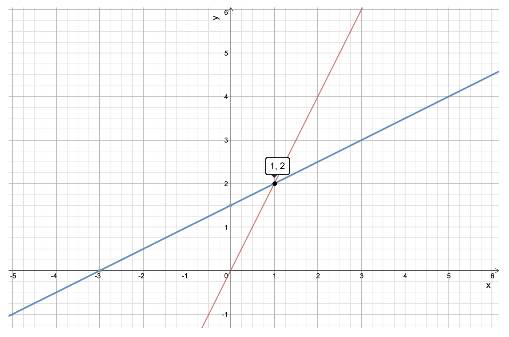
Column picture - linear combination of columns

Follow the column we can rewrite the equations above as follows:

x [\begin{matrix} 2 \\ - 1 \end{matrix}] + y [\begin{matrix} - 1 \\ 2 \end{matrix}] = [\begin{matrix} 0 \\ 3 \end{matrix}]

We can interpret the above equation as linear combination of columns which are vectors in 2-D, and the + is overloaded for 2-D vector addition, as compared with scalar addition in row picture interpretation. The geometry is shown below.

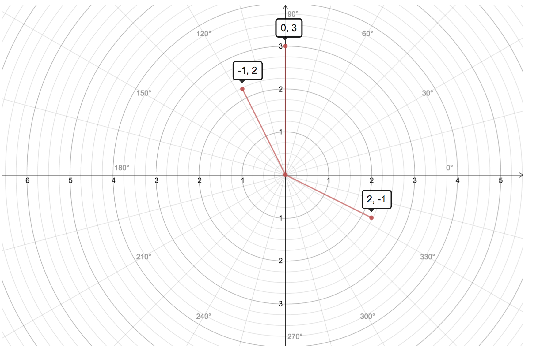
When considering high dimension problem (say n = 10, i.e., 10 linear equation with n unknowns), it is not easy to imagine n-D space from Row Picture. However from Column Picture, the result is just the linear combination of 10 vectors.

2. Matrix multiplication as linear combination

Usually we do matrix multiplication is to get the result cell as the dot product of a row in the first matrix with a column in the second matrix. However there is a very good interpretation from linear combination aspect, which is a core concept in linear algebra.

2.1 Linear combination of columns of matrix

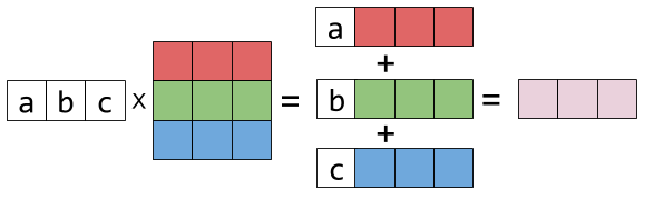
[\begin{matrix} 1 & 2 & 3 \\ 4 & 5 & 6 \\ 7 & 8 & 9 \end{matrix}] [\begin{matrix} a \\ b \\ c \end{matrix}] = a [\begin{matrix} 1 \\ 4 \\ 7 \end{matrix}] + b [\begin{matrix} 2 \\ 5 \\ 8 \end{matrix}] + c [\begin{matrix} 3 \\ 6 \\ 9 \end{matrix}] = [\begin{matrix} 1 a + 2 b + 3 c \\ 4 a + 5 b + 6 c \\ 7 a + 8 b + 9 c \end{matrix}]

Representing the columns of matrix by colorful boxes will help visualize this as follows: (the picture is from Eli Bendersky)

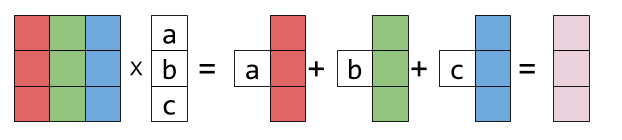
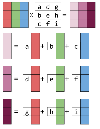
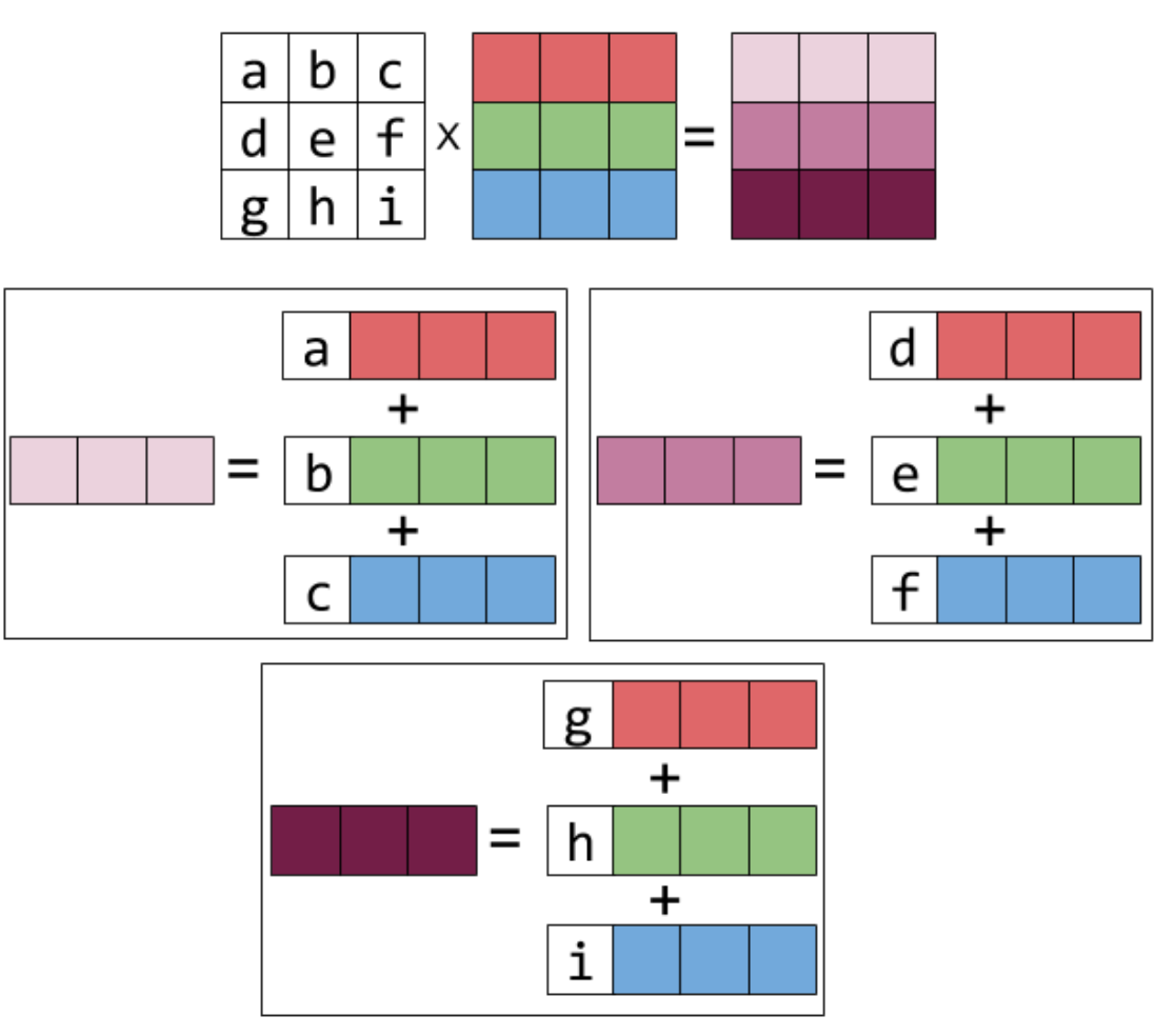
For matrix multiply a column vector, the result is a column vector which is the linear combination of the columns of the matrix and the coefficients are the second vector. This idea can also be generalized to Matrix-Matrix multiplication, i.e., the columns of the result matrix is the first matrix multiply each column (vector) in the second matrix respectively. The following picture shows the idea.

2.2 Linear combination of rows of matrix

Similarly we can view the matrix as different rows. $[\begin{matrix} a & b & c \end{matrix}] [\begin{matrix} 1 & 2 & 3 \\ 4 & 5 & 6 \\ 7 & 8 & 9 \end{matrix}] = a [\begin{matrix} 1 & 2 & 3 \end{matrix}] + b [\begin{matrix} 4 & 5 & 6 \end{matrix}] + c [\begin{matrix} 7 & 8 & 9 \end{matrix}]$ The above equation can be represented as follows:

For matrix-matrix multiplication, the rows of the result matrix is each row (vector) in first matrix multiply the second matrix. The idea can be represented graphically following:

2.3 Column-row multiplication

There is another interpretation of matrix multiplication from $c o l u m n * r o w$ view.

[\begin{matrix} a \\ b \\ c \end{matrix}] [\begin{matrix} x & y & z \end{matrix}] = [\begin{matrix} a x & a y & a z \\ b x & b y & b z \\ c x & c y & c z \end{matrix}]

The above result is a 3 by 3 matrix. And if we two matrix are m by n and n by p, the shape of the result matrix is m by p and the result is the sum of all the matrix (m by p) computed by all the $n^{t h}$ column in the first matrix and $n^{t h}$ row in the second matrix.

2.4 Block matrix multiplication

There is even another amazing interpretation of matrix multiplication. It is often convenient to partition a matrix A into smaller matrices called blocks. Then we can treat the blocks as matrix entries when do matrix multiplication.

A B = [\begin{array}{cc} a_{11} & a_{12} \\ a_{21} & a_{22} \end{array}] \cdot [\begin{array}{cc} b_{11} & b_{12} \\ b_{21} & b_{22} \end{array}] = [\begin{array}{cc} a_{11} b_{11} + a_{12} b_{21} & a_{11} b_{12} + a_{12} b_{22} \\ a_{21} b_{11} + a_{22} b_{21} & a_{22} b_{12} + a_{22} b_{22} \end{array}]

which is equal to:

A B = [\begin{array}{cc} A_{11} & A_{12} \\ A_{21} & A_{22} \end{array}] \cdot [\begin{array}{cc} B_{11} & B_{12} \\ B_{21} & B_{22} \end{array}] = [\begin{array}{cc} A_{11} B_{11} + A_{12} B_{21} & A_{11} B_{12} + A_{12} B_{22} \\ A_{21} B_{11} + A_{22} B_{21} & A_{22} B_{12} + A_{22} B_{22} \end{array}]

2.5 Elimination matrices

The linear combination interpretation of matrix multiplication is very useful for us to understand matrix transformation. Especially when we do row operation, we can achieve elimination to solve a system of linear equations. Take the following matrix multiplication for example AX=B, we want to choose the first matrix A in order to transform matrix X to B.

[\begin{matrix} a & b & c \\ d & e & f \\ g & h & i \end{matrix}] [\begin{matrix} 1 & 2 & 3 \\ 4 & 5 & 6 \\ 7 & 8 & 9 \end{matrix}] = [\begin{matrix} 1 & 2 & 3 \\ 0 & - 3 & - 6 \\ 7 & 8 & 9 \end{matrix}]

Recall that the row in result matrix the row in A multiply X, which is the linear combination of rows of X. Because the first and third row is the same, so the first and third row in A should be $[1 0 0]$ and $[0 0 1]$ and the second row in B is the second row minus 4 times first row in A, i.e., $[r o w 2 - 4 * r o w 1]$ . So the second row in A should be $[- 4 1 0]$ . Put all together A = $[\begin{matrix} 1 & 0 & 0 \\ - 4 & 1 & 0 \\ 0 & 0 & 1 \end{matrix}]$

2.6 Permutation of matrix

Exchange the two rows in a matrix A, we just need to multiply some matrix on the left as shown as follows. For example in the result matrix, the first row is the linear combination of the rows in the second matrix with respect to first row in the first matrix. What we want is the second row, so the second cell in the first matrix should be 1, and first cell should be 0, which has no contribution to the first row in the result matrix.

[\begin{matrix} 0 & 1 \\ 1 & 0 \end{matrix}] [\begin{matrix} a & b \\ c & d \end{matrix}] = [\begin{matrix} c & d \\ a & b \end{matrix}]

If want to exchange the columns, we just need to do column operation:

[\begin{matrix} a & b \\ c & d \end{matrix}] [\begin{matrix} 0 & 1 \\ 1 & 0 \end{matrix}] = [\begin{matrix} b & a \\ d & c \end{matrix}]

In short, if we want to do column operations the matrix multiplies on the right, and to do row operations, it multiplies on the left.

##3 Inverse or non-singular matrix Suppose A is square matrix, and if $A A^{- 1} = I$ ( $I$ is identity matrix), then matrix A is invertible and the inverse matrix is $A^{- 1}$ . We can see whether inverse matrix is a property for a given matrix, and not all matrices have inverse matrix. One simple way to determine whether you can find a vector x != 0 with Ax = b, and if you cannot find a x, then A has inverse matrix, otherwise not. For example,

[\begin{matrix} 1 & 3 \\ 2 & 6 \end{matrix}] [\begin{matrix} 3 \\ - 1 \end{matrix}] = [\begin{matrix} 0 \\ 0 \end{matrix}]

There couldn’t be an inverse for the first matrix above. We can think that the first and second column (vector) are in same direction, the linear combination of them can not be 0.

If matrix A does has inverse matrix, then Guass-Jordan elimination can solve it: $E [A I] = [I A^{- 1}]$ , where $E A = I$ . You interpret the equation as block matrix multiplication. We can use inverse matrix to factorize matrix as two matrix multiplication. First use elimination (or elemental) matrix E to transform A into U, i.e. $E A = U$ , then solve A as $A = E^{- 1} U = L U$ . The factors L and U are triangular matrices. Because of U is the result of elimination, so it should be a upper triangular matrix. For L, we can use Guass-Jordan elimination $E [A I] = [I A^{- 1}]$ to compute the L, because the we just do elimination of I with E, so the cell values in the upper bound are all zero, so L is a lower triangular matrix. If we need to exchange rows, all we need is to multiply a permutation matrix on the left: $P A = E^{- 1} U = L U$ .

Another property of invertible square matrix is that you can exchange transposing and inversing for a singular matrix. $(A^{- 1})^{T} A^{T} = I$ , i.e., $(A^{- 1})^{T} = (A^{T})^{- 1}$ . More more interesting thing is that when a matrix multiply its transpose, we get a symmetry matrix. $(A A^{T})^{T} = (A^{T})^{T} A^{T} = A A^{T}$ .

3. Vector Spaces

Vector space means the “space” of vectors, which should satisfy some rules, i.e., we can multiply any vector v by any scalar c in that space, that’s to say they can produce linear combination. For example, $R^{2}$ space contains all the real vectors with 2 components and it represents x-y plane, and $R^{2}$ space contains all the real vectors with 2 components and it represents x-y plane, and $R^{3}$ space contains all the real vectors with 3 components and it represents x-y-z 3-d space.

Subspace is a vector space which contains some or all the vectors from another vector space. Subspace should be satisfy the definition of space (linear combination) and it is based on another vector space. For instance, there are 4 subspace of $R^{3}$ : Z – the single vector (0 0, 0); (L) – any line through (0, 0, 0); (P) – any plane through(0, 0, 0); $R^{3}$ – the whole space.

In return, we can use some vectors or a matrix to construct vector space because all we need is linear combination. Given a matrix, the linear combination of all the columns of matrix from a space, which is called column space. For example:

A = [\begin{matrix} 1 & 2 \\ 3 & 4 \\ 5 & 6 \end{matrix}]

The column vector of A is in $m a t h b b R^{3}$ , and all the combinations of columns form a subspace, which is plane through origin. And the intersection of two subspace is a subspace.

##4. Interpret $A x = b$ with vector space #### column space We can interpret $A x$ (A is a matrix and x is a vector) as linear combination of columns of matrix using vector x, i.e., which is the columns space define by matrix A. So we can view $A x = b$ as finding the perfect linear combination of the columns to make it equal to vector b, and the vector b should be in the column space defined by matrix A.

A x = [\begin{matrix} 1 & 5 & 6 \\ 2 & 6 & 8 \\ 3 & 7 & 10 \\ 4 & 8 & 12 \end{matrix}] [\begin{matrix} x \\ y \\ z \end{matrix}] = b

Take above equation for example, not for all b we can find a solution. Because b could be any vector in $R^{4}$ and the left hand side the combinations of 3 columns don’t fill the whole 4-D space. The fact is that there are a lot of vectors b are not the combinations of the 3 columns (column subspace which is inside $m a t h b b R^{4}$ ). We can only solve the equation when b is in the column space of A, for example, $x = [1 0 0]^{T}$ , when $b = [1 2 3 4]^{T}$ .

Null space

Particularly for equation $A x = b = 0$ , we can get a bunch of vectors x as the solutions and this vectors can compose a subspace because $A (v + w) = A v + A w = 0$ . Take example above (when b = 0), the solution is $c [1 1 - 1]^{T}$ (c is constant), which is called Null space. And if $b! = 0$ , then the solution is not a subspace because 0 is not in that bunch of vectors.

5. Compute $A x = b$

Null space b = 0

We can do elimination for matrix A and get the matrix U, and then continue simplifying the U to get matrix R which is reduced row echelon form and R has the form of

[\begin{matrix} I & F \\ O & O \end{matrix}]

$I$ is identity matrix and indicates pivot variables. In fact the particular solutions are the columns of matrix $N = {[\begin{matrix} - F & I \end{matrix}]}^{T}$ , the null space is the column space of N. This is because of following matrix block multiplication.

[\begin{matrix} I & F \\ O & O \end{matrix}] [\begin{matrix} - F \\ I \end{matrix}] = O

b != 0

First we should consider whether the equation has solution or not, as mentioned above, Ax = b is solvable when b is column space of A, i.e., C(A). On the other hand, after finishing the elimination step, if the a combination of rows of A gives zero rows, the same combination of entries of b must give 0.

If the equation does have solutions, we can use elimination to find a particular solution. As long as we get one particular solution, the complete solution is the particular solution plus the any vector in the null space of A. that’s to say, $x = x_{p a r t i c u l a r} + x_{n u l l}$ . The shape of the complete solution is similar to Null space, we can interpret the complete space as null space which is shifted by vector $x_{p a r t i c u l a r}$ . This is because:

A x_{p} = b a n d A x_{n} = 0 = A (x_{p} + x_{b}) = b

Solution discussion – m by n matrix A of rank r

Full column rank, i.e., r = n

There are free variables
The null space is {0}
Unique solution if it exists (0 or 1 solution)
The reduced row echelon form is $[\begin{matrix} I \\ O \end{matrix}]$ .

Full row rank, i.e., r = m

It can be solved Ax=b for every b, because every row have a pivot and no zero rows.
There are n - r free variables and there are infinite solutions.
The reduced row echelon form is $[\begin{matrix} I & F \end{matrix}]$

Full column and row rank, i.e., r = m = n

Invertible matrix of A
Unique solution
The reduced row echelon form is identity I.

Not full rank, i.e., r < m, and r < n

There are no solutions or infinite solutions
The reduced row echelon form is $[\begin{matrix} I & F \\ 0 & 0 \end{matrix}]$

6. Independent, span, basis dimension

Independent is used to describe the relation between vectors. Vectors $v_{1}, v_{2}, . . ., v_{n}$ are Independent if no linear combination gives zero vector (except the zero combination), i.e., $c_{1} v_{1} + c_{2} v_{2} + . . . + c_{n} v_{n}! = 0$ . From vector space point of view, $v_{1}, v_{2}, . . ., v_{n}$ are columns of matrix A, they are independent if null space of A is zero vector and the rank r = n with no free variables, and they are independent if Ac = 0 for some non-zero vector c and rank < n with free variables.

Vectors $v_{1}, v_{2}, . . ., v_{n}$ span a vector space means that the space contains all the linear combination of those vectors. They vectors could be independent or dependent.

We are more interested in the vectors spanning a space are independent, which means the right number or minimal number of vectors to span a given space and we use basis to indicate this idea. Basis for a vector space is segment of vectors with 2 properties: (1) They are independent; (2)They span a space.

For a given space such as $R^{4}$ , every basis has the same number of vectors and the number is called dimension of the space. So when putting all together, we get the conclusion the rank of a matrix A == the number of pivot columns == dimension of the column space.

7. Orthogonal

Vector x is orthogonal to vector y, when $x^{T} y = 0$ Subspace S is orthogonal to subspace T means: every vector in S is orthogonal to every vector in T. For every space, the row space is orthogonal to nullspace. Because of Ax = 0, so the linear combination of rows respecting to null space is 0, i.e. $\sum_{i}^{m} c_{i} r o w_{i} = 0$ Moreover, nullspace and row space are orthogonal complements in $R^{n}$ and nullspace contains all vectors perpendicular to the row space.

8. “Solve” $A x = b$ when there are no solutions

We know that $A x = b$ is only solvable when vector b is in the column space of A. In practice, this equation is often unsolvable when A is a rectangular. Take m by n matrix (m n)for example, there are more constrains or equations than unknown variables and there may be no solutions when some equations conflict each other. In other words, there is a lot of information about x here. One naive method is only using some of information (equations), however, there is no reason to say some equations are perfect and some are useless and we want to use all the information to get the best solution.

When $A x = b$ cannot be solved perfectly, what can we do? And can we do better? The reason that the equation is not solvable is because b is not in the column space of A, so we may be able to find a “closest” vector (say p) to replace b in the column space of A, i.e., $A \hat{x} = p$ , and use $\hat{x}$ to estimate $x$ . The next problem is to define the “best” p, and the projection of b onto column space A is used instead. And then we need to find a way to calculate the projected vector p from b.

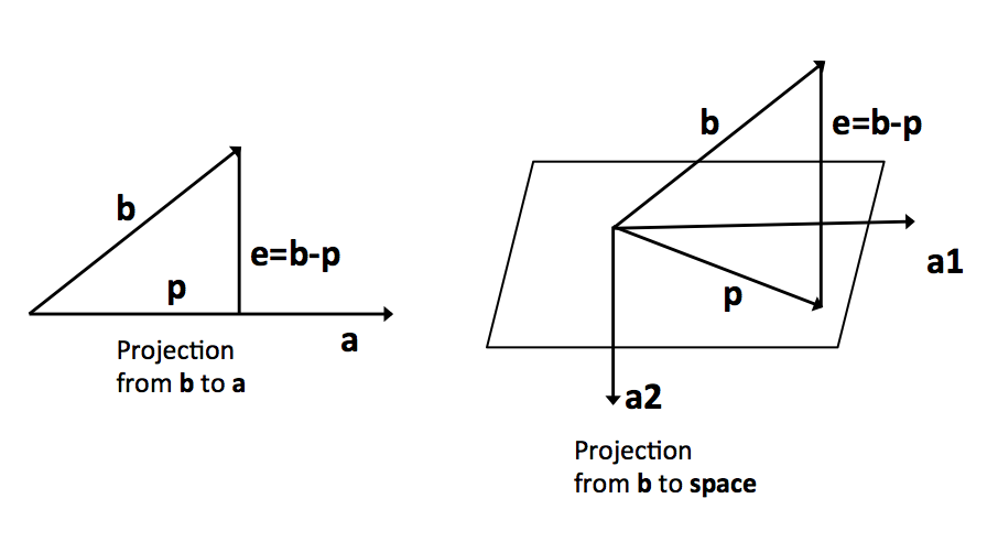
For simplicity, we first consider projection from vector to vector (see the left diagram above). We use p to indicate the projection of b onto a and b is equal to some multiple of a, i.e., $x a$ . According to is perpendicular to e, we have:

a^{T} e = a^{T} (b - x a) = a^{T} b - x a^{T} a = 0 = x = \frac{a^{T} b}{a^{T} a} S o p = x a = \frac{a^{T} b}{a^{T} a} a W e c a n r e w r i t e a s p = P b = (\frac{a a^{T}}{a^{T} a}) b

Notice that P is a n by n matrix if vector b and a have n elements and it is determined only by the vector a which we want to project onto. P is called projection matrix and we can interpret it as a function coming from vector a to project another vector to itself. Additionally we can observe that $P^{T} = (\frac{a a^{T}}{a^{T} a})^{T} = P$ and $P P = \frac{a a^{T}}{a^{T} a} \frac{a a^{T}}{a^{T} a} = \frac{a (a^{T} a) a^{T}}{(a^{T} a) (a^{T} a)} = P$

Next we consider projection from vector to space (see the right diagram above), the plane is the column space of A = [a1 a2], the error e = b - p and it is perpendicular to A. The projection b to A is $a_{1} x_{1} + x_{2} x_{2} = A x$ and our aim is to find x. Because e = b - Ax is perpendicular to the plane:

{\begin{cases} a_{1}^{T} (b - A x) = 0 \\ a_{2}^{T} (b - A x) = 0 \end{cases} = [\begin{matrix} a_{1}^{T} \\ a_{2}^{T} \end{matrix}] [\begin{matrix} b - A x \end{matrix}] = [\begin{matrix} 0 \\ 0 \end{matrix}] = A^{T} [\begin{matrix} b - A x \end{matrix}] = 0 = A^{T} b - A^{T} A x = 0 = x = (A^{T} A)^{- 1} A^{T} b = p = A x = A (A^{T} A)^{- 1} A^{T} b = P b

From above equation we can interpret the (b-Ax) is in the null space of $A^{T}$ , and the (b-Ax) should be perpendicular to the row space of $A^{T}$ which is the column space of A, which is the plane defined by a and b. The matrix $P = A (A^{T} A) - 1 A^{T}$ is called projection matrix, which can also be interpreted as a function to project a vector b onto the column space of A. Moreover $P^{T} = P$ and $P P = P$ . Here if A has independent columns then $A^{T} A$ is invertible. Here is a simple proof: suppose $A^{T} A x = 0$ , then x must be 0 if $A^{T} A$ is invertible.

A^{T} A x = 0 = x^{T} A^{T} A x = 0 = (A x)^{T} (A x) = 0 = A x = 0 = x = 0

9. Determinant

The square matrix is relatively easy to deal with, and the determinant is a number that associates with a square matrix, $d e t A = ‖ A ‖$ . Though this number can’t not tell you all the information of the matrix, it can tell you a lot of information. Following is some important properties of determinant.

Determinant of I is 1
Exchange two rows of a matrix: reverse sign of determinant.
Linear combination of one row, and det (A+B) != det(A) + det(B)

| \begin{matrix} t a & t b \\ c & d \end{matrix} | = t | \begin{matrix} a & b \\ c & d \end{matrix} | a n d | \begin{matrix} a + a^{'} & b^{'} + b \\ c & d \end{matrix} | = | \begin{matrix} a & b \\ c & d \end{matrix} | + | \begin{matrix} a^{'} & b^{'} \\ c & d \end{matrix} |

Two equal rows, then determinant is 0. We can get it by exchanging the same row.
Subtract l * row i from row k, and the determinant doesn’t change, i.e. elimination process.

| \begin{matrix} a & b \\ c - l a & d - l b \end{matrix} | = | \begin{matrix} a & b \\ c & d \end{matrix} | - l | \begin{matrix} a & b \\ a & b \end{matrix} | = | \begin{matrix} a & b \\ c - l a & d - l b \end{matrix} |

Row of zeros, the determinant is equal to 0
Triangular matrix, the determinant is product of pivots, which is based on property 3.
det A = 0, when A is singular, and det A != 0 when A is invertible.
det(AB) = det(A)*det(B), and $d e t (A^{- 1}) = \frac{1}{d e t (A)}$
$d e t (A^{T}) = d e t (A) | A^{T} | = | A | <= | U^{T} L^{T} | = | L U | <= | U^{T} | | L^{T} | = | L | | U |$

Cofactor of one entry Cofactor of $a_{i j} = c_{i} j$ is the (+/-) determinant of n-1 matrix with row i and column j erased, when i+j is even choose +, and choose - when i+j is odd. Cofactor formula is: $d e t (A) = a_{i 1} c_{i 1} + a_{i 2} c_{i 2} + . . . + a_{i n} c_{i n}$

Another very good interpretation is that the determinant is the volume of a box determined by row vectors.

10. Eigenvalue and eigenvector

The result vector $A x$ is parallel to x, and the vector x is called eigenvector of square matrix A, i.e.,

A x = λ x

The $λ$ is called eigenvalue.

A x = λ x = (A - λ I) x = 0

Notice that $(A - λ I)$ should be singular, otherwise x must be 0. So the det $(A - λ I)$ = 0, and after finding the eigenvalues we can find the eigenvectors by computing null space. For most n by n matrix, there are n eigenvectors and eigenvalues. Some matrix just has one eigenvectors and eigenvalues of some matrix are complex number.

Above we know how to compute the eigenvalues and eigenvectors, then how to use them. Suppose there are n independent eigenvectors of n by n matrix A, and put them in column matrix S.

A S = A [x_{1}, x_{2}, . . ., x_{n}] = [λ_{1} x_{1}, λ_{2} x_{2}, . . ., λ_{n} x_{n}] = [x_{1}, x_{2}, . . ., x_{n}] [\begin{matrix} λ_{1} & 0 & \dots & 0 \\ 0 & λ_{2} & \dots & 0 \\ 0 & 0 & ⋱ & 0 \\ 0 & 0 & \dots & λ_{n} \end{matrix}] = S Λ

$Λ$ is called diagonal eigenvalue matrix

A S = S Λ = S^{- 1} A S = Λ = A = S Λ S^{- 1}

In fact, the eigenvectors and eigenvectors give a way what is going on inside a matrix and to understand the power of matrix. For example, $A^{k} - 0 a s k - \infty$ if all $‖ λ_{i} ‖ < 1$ .

A x = λ x = A^{2} x = λ A x = λ^{2} x A^{2} = S Λ S^{- 1} S Λ S^{- 1} = S Λ^{2} S^{- 1} A^{k} = S Λ^{k} S^{- 1}

Base on the above equation, A is sure to have n independent eigenvectors and can be diagonalizable if all the eigenvalues $λ_{i}$ are different.

We can use eigenvectors to solve following problem: $u_{k + 1} = A u_{k}$ , start with a give vector $u_{0}$ , and we can see $u_{k} = A^{k} u_{0}$ . To really solve above equation, we can first write $u_{0}$ as the linear combination of eigenvectors of matrix A. Then:

u_{0} = c_{1} x_{1} + c_{2} x_{2} + . . . + c_{n} x_{n} = A u_{0} = A (c_{1} x_{1} + c_{2} x_{2} + . . . + c_{n} x_{n}) = c_{1} λ_{1} x_{1} + c_{2} λ_{2} x_{2} + . . . + c_{n} λ_{n} x_{n} = A^{2} u_{0} = A A u_{0} = A (c_{1} λ_{1} x_{1} + c_{2} λ_{2} x_{2} + . . . + c_{n} λ_{n} x_{n}) = c_{1} {λ_{1}}^{2} x_{1} + c_{2} {λ_{2}}^{2} x_{2} + . . . + c_{n} {λ_{n}}^{2} x_{n} = A^{k} u_{0} = c_{1} {λ_{1}}^{k} x_{1} + c_{2} {λ_{2}}^{k} x_{2} + . . . + c_{n} {λ_{n}}^{k} x_{n} = S Λ c

Using above idea to solve Fibonacci problem, [0, 1, 1, 2, 3, 5, 8, 13, …], then how to get $F_{1} 00$ . So we need to find how fast the sequence grows, which lies in the eigenvalues.

We want the form $u_{k + 1} = A u_{k}$ to use the matrix A. And we can construct the matrix as follows

{\begin{cases} F_{k + 2} = F_{k + 1} + F_{k} \\ F_{k + 1} = F_{k + 1} \end{cases} = u_{k + 1} = A u_{k} = [\begin{matrix} 1 & 1 \\ 1 & 0 \end{matrix}] u_{k} a n d u_{k} = [\begin{matrix} F_{k + 1} \\ F_{k} \end{matrix}] A = [\begin{matrix} 1 & 1 \\ 1 & 0 \end{matrix}] = | A - λ I | = λ^{2} - λ - 1 = λ_{1} = \frac{1 + \sqrt{5}}{2} \approx 1.618 λ_{2} = \frac{1 - \sqrt{5}}{2} \approx - 0.618 E i g e n v e c t o r s a r e x_{1} = [λ_{1} 1]^{T}, x_{2} = [λ_{2} 1]^{T} u_{0} = [1 0]^{T} = c_{1} x_{1} + c_{2} x_{2} = c_{1} = 0.447 c_{2} = - 0.447 u_{100} = A^{100} u_{0} = c_{1} {λ_{1}}^{100} x_{1} + c_{2} {λ_{2}}^{100} x_{2} = 0.447 (1.618)^{100} [1.618 1]^{T} - 0.477 (- 0.618)^{100} [- 0.618 1] u_{100} \approx 0.447 (1.618)^{100} [1.618 1]^{T}

11. First order differential equation $d_{u} / d_{t} = A u$

We also arrange two or more equation into matrix form and try to solve it from matrix aspect. For example:

{\begin{cases} \frac{d u_{1}}{d t} = - u_{1} + 2 u_{2} \\ \frac{d u_{2}}{d t} = u_{1} - 2 u_{2} \end{cases} = \frac{d u}{d t} = A [\begin{matrix} u 1 \\ u 2 \end{matrix}] = [\begin{matrix} - 1 & 2 \\ 1 & - 2 \end{matrix}] [\begin{matrix} u 1 \\ u 2 \end{matrix}]

We can see from the above equation, u2 and u1 can be affected by each other and the relationship or all information, in fact, is the matrix A. So we maybe solve the differential equations as a single system. Usually this system is called Linear Dynamic System.

We can use eigenvectors and eigenvalues of matrix A to solve above system. The result is very simple $u (t) = e^{t A} u (0)$ . The key point is the matrix exponential, which can be interpreted by Taylor Series.

\begin{matrix} (1) & \begin{aligned} e^{A t} & = I + A t + \frac{(A t)^{2}}{2!} + \frac{(A t)^{3}}{3!} + . . . + \frac{(A t)^{n}}{n!} + . . . \\ = S I S^{- 1} + S Λ S^{- 1} t + \frac{S Λ^{2} S^{- 1} t}{2!} + \frac{S Λ^{n} S^{- 1} t}{n!} + . . . \\ = S (I + Λ t + \frac{Λ^{2} t}{2!} + \frac{Λ^{n} t}{n!} + . . .) S^{- 1} \\ = S e^{Λ t} S - 1 \end{aligned} \end{matrix}

In the above equation, the S and $Λ$ are defined by eigenvectors and eigenvalues. Notice that the equation should based on the fact that there are n independent eigenvectors of matrix A, i.e., A can be diagonalized. Moreover the $e^{Λ t}$ can be easily computed as follows:

\begin{matrix} (2) & \begin{aligned} e^{Λ t} & = I + Λ t + \frac{Λ^{2} t}{2!} + \frac{Λ^{n} t}{n!} + . . . \\ = I + {[\begin{array}{c} λ_{1} & 0 & \dots & 0 \\ 0 & λ_{2} & \dots & 0 \\ 0 & 0 & ⋱ & 0 \\ 0 & 0 & \dots & λ_{n} \end{array}]}^{1} + . . . + \frac{1}{n!} {[\begin{array}{c} λ_{1} & 0 & \dots & 0 \\ 0 & λ_{2} & \dots & 0 \\ 0 & 0 & ⋱ & 0 \\ 0 & 0 & \dots & λ_{n} \end{array}]}^{n} + . . . \\ = [\begin{array}{c} e^{λ_{1} t} & 0 & \dots & 0 \\ 0 & e^{λ_{2} t} & \dots & 0 \\ 0 & 0 & ⋱ & 0 \\ 0 & 0 & \dots & e^{λ_{n} t} \end{array}] \end{aligned} \end{matrix}

12. Symmetric matrix and positive definite

Symmetric matrix is very special matrix and they are good matrices: the eigenvalues are REAL and eigenvectors can be chosen PERPENDICULAR. For usual case $A = S Λ S^{- 1}$ , for symmetric matrix $A = Q Λ Q^{- 1} = Q Λ Q^{T}$ , and the matrix Q is the orthonormal eigenvectors matrix.

In additional, $A = Q Λ Q^{T} = \sum_{i}^{n} λ_{i} q_{i} {q_{i}}^{T}$ , so every symmetric matrix is a combination of perpendicular projection matrices. This is because $q_{i} {q_{i}}^{T} = \frac{q_{i} {q_{i}}^{T}}{q_{i}^{T} q_{i}}$ , which is projection matrices.

Then how about the sign of $λ_{i}$ , and the eigenvalues decides between instability and stability in differential equations. Positive definite means that all the eigenvalues are positive. Positive semidefinite is called when eigenvectors are greater or equal to zero. Formally the Positive definite of matrix A is defined as the quadratic form is greater that zero, i.e., $x^{T} A x 0$

x^{T} A x = [\begin{matrix} x & y \end{matrix}] [\begin{matrix} a & b \\ c & d \end{matrix}] [\begin{matrix} x \\ y \end{matrix}] = a x^{2} + (b + c) x y + d y^{2}

Another fact is that the signs of pivots are the same as signs of $λ_{i}$ and the number of positive pivot is equal to the number of positive eigenvalues.

We can interpret the quadratic form $x^{T} A x = 1$ as tiled ellipse associated with symmetric matrix A. $X^{T} Λ X = 1$ is a lined-up ellipse associated with eigenvalues matrix $L a m b d a$ , and we can use eigenvectors matrix Q to rotate the tiled ellipse to lined-up ellipse. Here is an example:

5 x^{2} + 8 x y + 5 y^{2} = 1 = [\begin{matrix} x & y \end{matrix}] A [\begin{matrix} x \\ y \end{matrix}] = [\begin{matrix} x & y \end{matrix}] [\begin{matrix} 5 & 4 \\ 4 & 5 \end{matrix}] [\begin{matrix} x \\ y \end{matrix}]

Use eigenvectors and eigenvalues to diagonalized $A = Q Λ Q^{T}$

[\begin{matrix} 5 & 4 \\ 4 & 5 \end{matrix}] = \frac{1}{\sqrt{2}} [\begin{matrix} 1 & 1 \\ 1 & - 1 \end{matrix}] [\begin{matrix} 9 & 0 \\ 0 & 1 \end{matrix}] \frac{1}{\sqrt{2}} [\begin{matrix} 1 & 1 \\ 1 & - 1 \end{matrix}]

So $5 x^{2} + 8 x y + 5 y^{2} = 9 (\frac{x + y}{\sqrt{2}})^{2} + 1 (\frac{x - y}{\sqrt{2}})^{2} = 9 X^{2} + 1 (Y)^{2} = 1$ . We can see that the axes of the titled ellipse point are along the eigenvectors and the axis lengths are determined by eigenvalues, i.e. $\frac{1}{\sqrt{λ_{i}}}$

So in the xy system, the axes are along he eigenvectors of A. In the XY system, the axes are along the eigenvectors of $Λ$ . So if $A = Q Λ Q^{T}$ is positive definite, i.e., $Λ_{i} 0$ . The graph $x^{T} A x = 1$ is an ellipse:

[\begin{matrix} x & y \end{matrix}] Q Λ Q^{T} [\begin{matrix} x \\ y \end{matrix}] = [\begin{matrix} X & Y \end{matrix}] Λ [\begin{matrix} X \\ Y \end{matrix}] = λ_{1} X^{2} + λ_{2} Y^{2} = 1.

$A = Q Λ Q^{T}$ is called the principal axis theorem, which can help displays the axes, or rotate to a lined-up position.

Singular value decomposition (SVD)

For a full rank square matrix, we can diagonalize the matrix as $S^{- 1} A S$ . However, if A is any m by n matrix with rank r, can we still diagonalize it?

Based on the symmetric matrix, suppose A can be diagonalized as $A = U Σ V^{T}$ , U and V are orthonormal matrix, $Σ$ is a diagonal matrix. The idea in fact is very simple, that’s we make A to be symmetric matrix.

A^{T} A = V Σ^{T} U^{T} U Σ V^{T} = V Σ^{2} V^{T} = Q_{1} Λ Q_{1}^{T} A A^{T} = U Σ V^{T} V Σ^{T} U^{T} = U Σ^{2} U^{T} = Q_{2} Λ Q_{2}^{T}

Because $A^{T} A$ and $A A^{T}$ are symmetric matrix, we easily get V, U and $Σ$ . In details, $v_{1}, . . . v_{r}$ are orthonormal singular vectors in row space of A, the $u_{1}, . . ., u_{r}$ are orthonormal simple vectors in column space. We need n-r more v’s and m-r u’s from the null space N(A) and left null space $N (A^{T})$ , $V v_{n} = 0 v_{m}$ , and we set $σ_{i} = 0$ when i r.

A [v_{1}, . . ., v_{r}, . . ., v_{n}] = [u_{1}, . . ., u_{r}, . . ., u_{m}] [\begin{matrix} σ_{1} & 0 & \dots & 0 \\ 0 & σ_{r} & \dots & 0 \\ 0 & 0 & ⋱ & 0 \\ 0 & 0 & \dots & 0 \end{matrix}]

9. Reference and further reading

Introduction to Linear Algebra from MIT OpenCourseWare