Support Vector Machine

Support vector machine (SVM) is often considered one of the best “out of the box” classifiers, and in this post I try to explain how we can come up with this algorithm from scratch.

I also implement the SMV for image classification with CIFAR-10 dataset by Python (numpy). This is for mutli-classification by using SVM loss.

1. Problem setting

Classification problem is to classify different objects into different categories. For simplicity, we just focus on binary classification that y can take two values 1 or -1 (indicating two classes), and we firstly assume the two classes are linearly separable. After all, it is reasonable to solve problems from simple to complex.

2. Basic idea (What we have known)

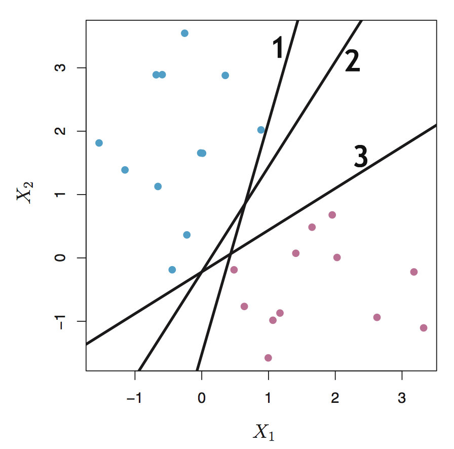
If the data is linearly separable, our goal is to find the such a line \(f(x) = w^Tx + b = 0\) (2-dimension) that divides the plane into 2 parts and each part represent one class (see following figure). If the data is represented in high dimension say N-dimension, what we need to do is to find a hyperplane \(w^Tx + b = 0\) which is subspace with dimension (N-1)dimension. So if \(w^Tx + b = 0\), the label \(y = 1\), otherwise \(y = -1\). However, the problem is that in fact there exists infinite such hyperplanes if the data can be perfectly linearly separated, because a given separating hyperplane can be shifted a tiny bit up or down, or rotated without coming into contact with any of the observations (the line 1, 2 and 3 in the following figure) . Of course we can randomly choose a separating line.

3. Maximal Margin Classifier

Can we do better?

Is that possible for us to choose the even “best” line or hyperplane from the infinit possible separating hyperplanes? So the next question is how to define the “best” hyperplane. Because the final goal is trying to use the hyperplane as decision boundary to distinguish the two classes, so we can choose the hyperplane which can make the distinction more obvious. Intuitively the separating hyperplane should be farthest from the training observations, that’s to say, the distance between the nearest observation and the hyperplane should be maximized. This distance is usually called margin and the corresponding classifier is known as maximal margin classifier, and the separating hyperplane has the farthest minimum distance to the training observations. Take the above figure for example, line 3 is better than line 1 and 2.

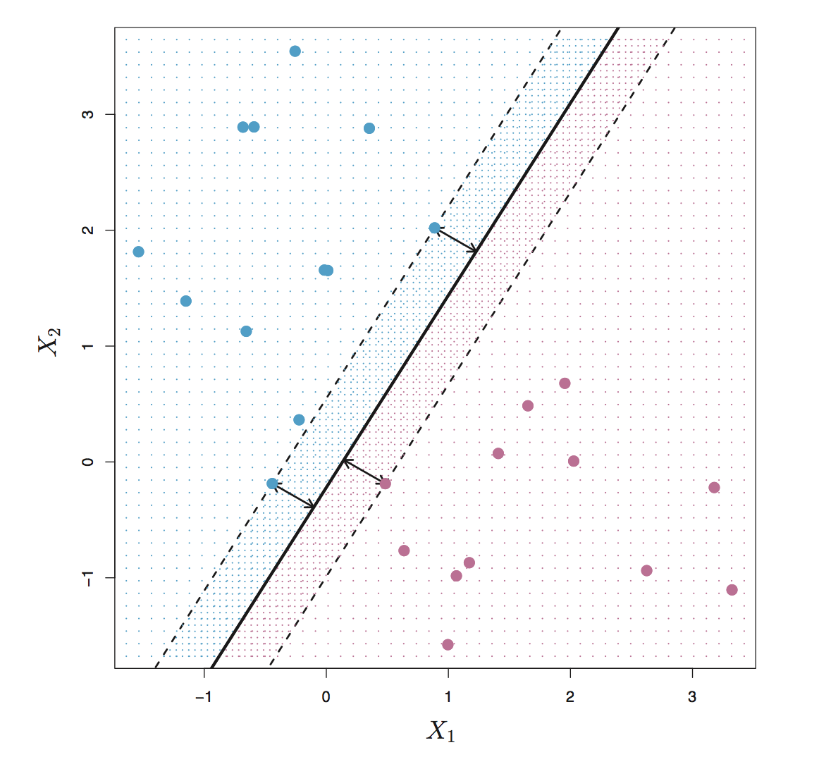
From figure below, we can see that there are 3 training points having equal distance from the maximal margin line and the two dash lines indicate the width of margin. These 3 observations are known as support vectors. Since these points can interpreted as n-1 dimension vectors and define the maximal margin, in other words, these vectors can “support” the maximal margin hyperplane in the sense that if these points were moved slightly then the maximal margin hyperplane would move as well. What’s more, the maximal margin hyperplane is only depends on the support vectors, not other observation.

Calculate the maximal margin In order to calculate the maximal margin, we should figure out how to calculate the geometric margin which is the distance from a point to a line or hyperplane. As following figure, the point at A representing the input \(x^{(i)}\) of some training example. Its distance to the decision boundary (a line with (w, b)) is \(\gamma^{(i)}\), is given by the line segment AB. And the distance \(\gamma^{(i)}\) can be calculate in the following way:

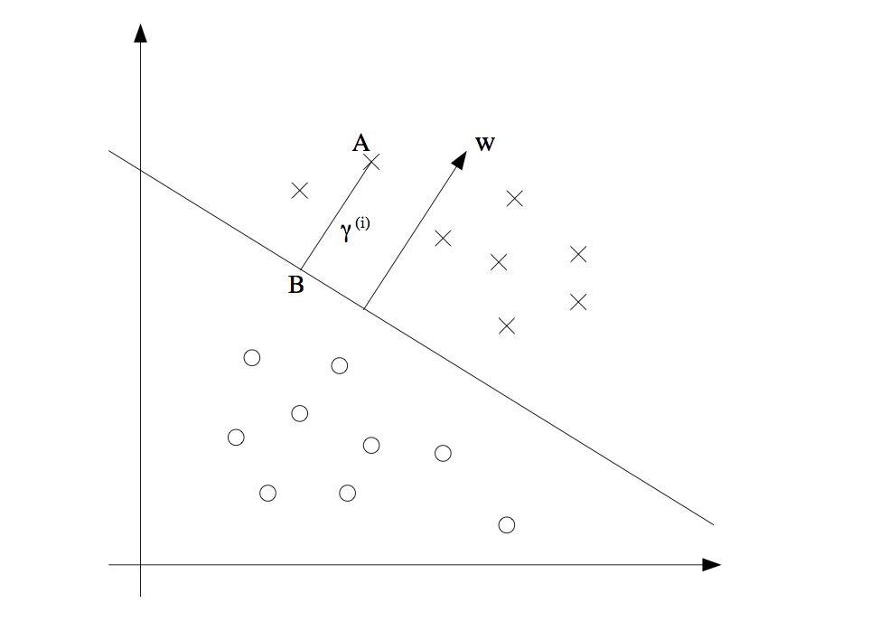
vector \(BA = x_A - x_B\), unit vector is \(w/\|w\|\), so the point B is given by \(x^{(i)} - \gamma^{(i)} w/\|w\|\). And point B is on the decision boundary \(w^T x + b\), therefore

Then solving \(\gamma^{(i)}\) yields:

Using bias trick to represent the two parameters w and b as one, i.e. set \(x_0 = 1\) and add \(w_0\) to weights vector w. Then we get:

Therefore based on a set of m training observations \(x_1, x_2, ..., x_m\) and associated class labels \(y_1, y_2, ..., y_m \in \big\{1, -1\big\}\), the assumption that the training set is linearly separable, the maximal margin line or hyperplane is the solution to the optimization problem.

Subject to

The constrains (2) guarantees that each observation will be on the correct side of the decision boundary and the value of \(y^{(i)} (W^Tx^{(i)})\) is at least M, provided that M is positive. In addition, the margin is given by \(\frac{w^T x^{(i)}}{\|w\|}\), the objective function \((1) \frac{M}{\|w\|}\) ensures that each observation has at least a distance \(\frac{M}{\|w\|}\) from the hyperplane or decision boundary. Hence, the optimization problem choose w and M to maximize \(\frac{M}{\|w\|}\).

Solve the optimization problem

If we could solve the optimization problem above efficiently, then we would be done. In fact the optimization problem above is very difficult because we have a nasty objective \(\frac{M}{\|w\|}\) function, which is non-convex. So can we do better?

The final goal is to find the decision boundary \(w^T x = 0\), so multiplying w by some constant can affect the margin but doesn’t change the decision boundary. Therefore, we can set the value of \(w^T x_0\) for the nearest point to be 1, i.e., \(M = 1\). Additionally maximize \(\frac{1}{\|w\|}\) is the same to minimize |w|, again is the same thing as minimizing \(\|w\|^2\). Therefore we have the following optimization problem:

Subject to

The new version of optimization problem can be efficiently solved, because the objective function is a convex quadratic function and all the constrains are linear. The problem can be solved by Quadratic Program (QR) software such as CVXOPT for Python.

4 Dual Form, Kernel and Support Vector Machine

According to Lagrange duality, we can get the dual form of the above optimization problem.

Subject to

The \(\langle x^{(i)}, x^{(j)}\rangle = \big(x^{(i)}\big)^T x^{(j)}\), and the original w = \(\sum_i^m \alpha_i y^{(i)}x^{(i)}\). And the decision boundary becomes

Therefore, we can solve the dual problem (optimizing the \(\alpha\)) in lieu of solving the primal optimization problem. Specifically in order to ake a prediction, all we need to do is to calculate the inner product between the new point x and each of the training samples \(x_i\). However, it turns out that \(\alpha_i's\) will be zero except for the support vectors, so we only need to find the inner products between x and support vectors to make prediction.

So far, what we’ve got is just a linear classifier or linear boundary \(w^T x + b = 0\). And if we want a non-linear boundary, what we can do? Intuitively we can use non-linear items in the boundary functions such as \(wx^2\) and \(wx^3\). In general we need to use a non-linear function (g(x)) to transfer the original input x to a new value g(x) which are passed into learning algorithm. These new quantities are often called features and the original input x can be called attributes. Usually people use \(\phi(x)\) the feature mapping, which maps from attributes to features. Here is a example:

Then the decision boundary is \(f(x) = w_1 x + w_2 x^2 + w_3 x^3 + b = 0\)

We should notice that the above decision boundary is a non-linear in 2-dimension space, i.e., \(w_1 x + w_2 x^2 + w_3 y + b = 0\), however we get a plane in a 3-dimension space \(w_1 x + w_2 y + w_3 z + b = 0\), which we can be solved by using maximal classifier discussed above.

Thus, rather than using the original input attributes x, we may instead use the features \(\phi(x)\). To do so, we just need to change the previous algorithm by replacing x with \(\phi(x)\).

The next question is how to choose the feature mapping, and we could choose arbitrary non-linear functions to compute features \(\phi(x)\), and then calculate the inner product of \(\phi(x)^T \phi(z)\). However, it may be very expensive to compute the features and the inner product when features are high dimension vectors.

One important property of the dual form is that the algorithm can be written entirely in terms of inner product \(\langle x, z\rangle\), which means that we can replace the inner product with \(\langle \phi(x), \phi(z) \rangle\). And we define the Kernel as following:

The goal is to compute the \(K(x, z)\), and the interesting is that \(K(x, z)\) may be not expensive to calculate because we don’t firsly need to compute the \(\phi(x)\) and then calculate the inner product (see following example).

Suppose the \(x, z \in \mathbb{R}^n\) and we can can construct the Kernel:

We can rewrite it as following

We can see \(K(x, z) = \phi(x)^T \phi(z)\), where the \(\phi(x)\) is shown below (take n = 3)

So we can efficiently calculate the \(K(x, z) = (x^T z)^2\) in \(O(n)\) because of n-dimension input attributes x. However, it takes \(O(n^2)\) to calculate \(\phi(x)\).

In general, we can also use \(K(x, z) = (X^T z + c)^d\) to achieve feature mapping, which is known as ploynomial kernel of degree d. This kernel essentially amount to fitting a support vector classifier in a higher-dimensional space involving polynomials of degree d, which leads to a much more flexible decision boundary. Notice that though working in a very high dimension space, we only need \(O(n)\) time to compute the K(x, z) because we never need to explicitly represent feature vectors in the very high dimensional feature space.

Another popular choice is Gaussian Kernel or Radial Kernel:

We can use Taylor expansion to expand the Gaussian Kernel (\(e^x = \sum_{n=0}^\infty \frac {x^n} {n!}\)), and we can see that the feature vector that corresponds to the Gaussian kernel has infinite dimensionality, and the feature space is implicit.

How does the Kernel work? One intuition is to think of \(K(x, z)\) as a measurement of how similar are \(\phi(x)\) and \(\phi(z)\), or of how similar are x and z. If \(\phi(x)\) and \(\phi(z)\) are close to each other, then \(K(x, z) = \phi(x)^T \phi(z)\) is expected to large, otherwise \(\phi(x)\) and \(\phi(z)\) are far apart, then \(K(x, z)\) is small. Recall that we use the sign of

for prediction. Look at Gaussian Kernel, if training observations that are far from test observation x will play essentially little role in the predicted class label for x. This means that Gaussian Kernel has a local hehavior, in the sense that only nearby training observations have a big effect on a class label for test observation.

The Support Vector Machine is an extension of the support vector classifier that results from enlarging the feature space in a specific way, using kernels.

5 The Non-separable Case

The SVMs work very well for classification if a separating hyperplane exists, however, we will get stuck when the data is overlapped and non-separable because there is no max margin. So we can extend the separating hyperplane in order to almost separate the classes based on soft margin. We instead allow some observations to be on the incorrect side of the margin, or even the incorrect side of the hyperplane. We reformulate the optimization problem as follows:

Subject to

Thus, we permit the observation to be on the incorrect side of the margin, or even the incorrect side of the hyperplane (\(1-\zeta_i < 0\)), and we pay a cost of the objective function being increased by \(C\zeta_i\). The big number C ensuring that \(\zeta_i\) is small and most examples have at least soft max margin.

And the dual form is as follows:

Subject to

Above is the basic idea of Support Vector Machine (SVM), all that remains is to to find a algorithm for solving the dual problem. The SMO (sequential minimal optimization) algorithm give an efficient way to solve the dual problem. You can find the details here.

6 Multiclass classification

We need to generalize to the multiple class case, that’s to say, the value of y is not binary any more, instead y can equal to 0, 1, 2, …, k.

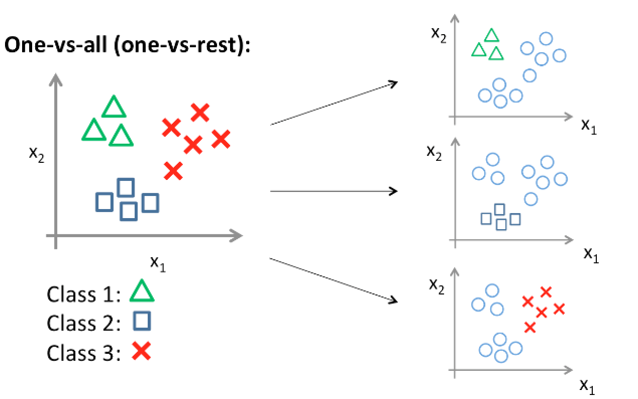
####Transfer multi-class classification into binary classification problem

We need change multiple classes into two classes, and the idea is to construct several logistic classifier for each class. We set the value of y (label) of one class to 1, and 0 for other classes. Thus, if we have K classes, we build K SVM and use it for prediction. The idea is the same as use logistic regression for multi-classification.

Multi-class Support Vector Machine loss

Similar to softmax, For mutilple classes problems (K categoires), it is possible to establish a mapping function for each class. We can simply use a linear mapping for all classes (K mapping function):

Intuitively we wish that the correct class has a score that is higher than the scores of incorrect classes. Thus, we can predict the test observation as the class with the highest score. Next we should find a loss function to optimize the parameters.

For sample \(x_i\), the vector \(f(x_i, W)\) is the scores for all the classes, \(y_i\) is the correct class and \(f(x_i, W)_{y_i}\) is the score corresponding to the correct class for \(x_i\). The score for the \(j^{th}\) class is \(f(x_i, W)_j\). The multiclass SVM loss for the \(i^{th}\) sample is as follows:

Though the expression seems complex, the interpretation is relatively simple. Firstly every class contribute to the loss of one sample, and the correct class doesn’t lead to loss. We want the correct class for sample \(x_i\) have a score \(f(x_i, W)_{y_j}\) higher than the incorrect classes \(f(x_i, W)_j\) by some fixed margin. If the incorrect class score adds some fix margin still less than correct class score, i.e., \(f(x_i, W)_j + \Delta < f(x_i, W)_{y_j}\), then set the loss to be zero. Because the correct score is “much” big than than the incorrect scores, which we desire to achieve. However, if the the correct class score is not “big” enough or even less than the incorrect class scores, then we set the loss to be \(f(x_i, W)_j + \Delta - f(x_i, W)_{y_j}\). Additionally the function max(0, -) is often called the hinge loss.

We still need regularization to our loss function. Suppose that we’ve got a set of weights W that can correctly classify all the samples, then the set of W is not necessarily unique. Firstly if we multiply a number \(\lambda\) W, then the decision boundary remains the same. So the scores stretches accordingly but the magin \(\Delta\) doesn’t change. Usually people add \(L_2\) regularization penalty R(W) to loss function.

So the full loss is as follows:

When \(\lambda\) is big, then \(R(W) = \sum_k \sum_l W_{k, l}^2\) is small. From binary SVM above, we know that the distance between one observation and the hyperplane of correct class is \(\frac{f(x_i, W)_{y_j}} {\|w_{k}\|}\). therefore, the \(L_2\) penalty leads to the max margin property in SVMs and improve the generalization of the performance of the classifiers and avoid overfitting.

This loss function has no constrains and we can calculate the gradient and optimize the W using gradient descent algorithm. For single example the SVM loss is:

We can differentiate the function with respect to weights. For w corresponding to the correct class:

The gradient for incorrect class:

where \(\mathbb{1}\) is the indicator function that is one if the condition is true or zero otherwise.

7 Get your hands dirty and have fun

• Purpose: Implement multi-classification classifier.
• Data: CIFAR-10 dataset, consists of 60000 32x32 colour images in 10 classes, with 6000 images per class. There are 50000 training images and 10000 test images. The data is available here.
• Setup: I choose Python (IPython, numpy etc.) on Mac for implementation, and the results are published in a IPython notebook.
• click here for the implementation.
• Following is code to implement the logistic, one-vs-all and softmax classifiers by gradient decent algorithm.

classifiers: algorithms/classifiers.py

import numpy as np
from algorithms.classifiers.loss_grad_logistic import *
from algorithms.classifiers.loss_grad_softmax import *
from algorithms.classifiers.loss_grad_svm import *

class LinearClassifier:

    def __init__(self):
        self.W = None # set up the weight matrix 

    def train(self, X, y, method='sgd', batch_size=200, learning_rate=1e-4,
              reg = 1e3, num_iters=1000, verbose=False, vectorized=True):
        """
        Train linear classifier using batch gradient descent or stochastic gradient descent

        Parameters
        ----------
        X: (D x N) array of training data, each column is a training sample with D-dimension.
        y: (N, ) 1-dimension array of target data with length N.
        method: (string) determine whether using 'bgd' or 'sgd'.
        batch_size: (integer) number of training examples to use at each step.
        learning_rate: (float) learning rate for optimization.
        reg: (float) regularization strength for optimization.
        num_iters: (integer) number of steps to take when optimization.
        verbose: (boolean) if True, print out the progress (loss) when optimization.

        Returns
        -------
        losses_history: (list) of losses at each training iteration
        """

        dim, num_train = X.shape
        num_classes = np.max(y) + 1 # assume y takes values 0...K-1 where K is number of classes

        if self.W is None:
            # initialize the weights with small values
            if num_classes == 2: # just need weights for one class
                self.W = np.random.randn(1, dim) * 0.001
            else: # weigths for each class
                self.W = np.random.randn(num_classes, dim) * 0.001

        losses_history = []

        for i in xrange(num_iters):
            if method == 'bgd':
                loss, grad = self.loss_grad(X, y, reg, vectorized)
            else:
                # randomly choose a min-batch of samples
                idxs = np.random.choice(num_train, batch_size, replace=False)
                loss, grad = self.loss_grad(X[:, idxs], y[idxs], reg, vectorized) # grad =[K x D]
            losses_history.append(loss)

            # update weights
            self.W -= learning_rate * grad # [K x D]
            # print self.W
            # print 'dsfad', grad.shape
            if verbose and (i % 100 == 0):
                print 'iteration %d/%d: loss %f' % (i, num_iters, loss)

        return losses_history

    def predict(self, X):
        """
        Predict value of y using trained weights

        Parameters
        ----------
        X: (D x N) array of data, each column is a sample with D-dimension.

        Returns
        -------
        pred_ys: (N, ) 1-dimension array of y for N sampels
        h_x_mat: Normalized scores
        """
        pred_ys = np.zeros(X.shape[1])
        f_x_mat = self.W.dot(X)
        if self.__class__.__name__ == 'Logistic':
            pred_ys = f_x_mat.squeeze() =0
        else: # multiclassification
            pred_ys = np.argmax(f_x_mat, axis=0)
        # normalized score
        h_x_mat = 1.0 / (1.0 + np.exp(-f_x_mat)) # [1, N]
        h_x_mat = h_x_mat.squeeze()
        return pred_ys, h_x_mat

    def loss_grad(self, X, y, reg, vectorized=True):
        """
        Compute the loss and gradients.

        Parameters
        ----------
        The same as self.train()

        Returns
        -------
        a tuple of two items (loss, grad)
        loss: (float)
        grad: (array) with respect to self.W
        """
        pass

# Subclasses of linear classifier
class Logistic(LinearClassifier):
    """A subclass for binary classification using logistic function"""
    def loss_grad(self, X, y, reg, vectorized=True):
        if vectorized:
            return loss_grad_logistic_vectorized(self.W, X, y, reg)
        else:
            return loss_grad_logistic_naive(self.W, X, y, reg)

class Softmax(LinearClassifier):
    """A subclass for multi-classicication using Softmax function"""
    def loss_grad(self, X, y, reg, vectorized=True):
        if vectorized:
            return loss_grad_softmax_vectorized(self.W, X, y, reg)
        else:
            return loss_grad_softmax_naive(self.W, X, y, reg)

class SVM(LinearClassifier):
    """A subclass for multi-classicication using SVM function"""
    def loss_grad(self, X, y, reg, vectorized=True):
        return loss_grad_svm_vectorized(self.W, X, y, reg)

Function to compute loss and gradients for SVM classification: algorithms/classifiers/loss_grad_svm.py

# file: algorithms/classifiers/loss_grad_svm.py
import numpy as np

def loss_grad_svm_vectorized(W, X, y, reg):
    """
    Compute the loss and gradients using softmax function 
    with loop, which is slow.

    Parameters
    ----------
    W: (K, D) array of weights, K is the number of classes and D is the dimension of one sample.
    X: (D, N) array of training data, each column is a training sample with D-dimension.
    y: (N, ) 1-dimension array of target data with length N with lables 0,1, ... K-1, for K classes
    reg: (float) regularization strength for optimization.

    Returns
    -------
    a tuple of two items (loss, grad)
    loss: (float)
    grad: (K, D) with respect to W
    """

    dW = np.zeros(W.shape)
    loss = 0.0
    delta = 1.0

    num_train = y.shape[0]

    # compute all scores
    scores_mat = W.dot(X) # [C x N] matrix
 
    # get the correct class score 
    correct_class_score = scores_mat[y, xrange(num_train)] # [1 x N]
    
    margins_mat = scores_mat - correct_class_score + delta # [C x N]

    # set the negative score to be 0
    margins_mat = np.maximum(0, margins_mat)
    margins_mat[y, xrange(num_train)] = 0

    loss = np.sum(margins_mat) / num_train

    # add regularization to loss
    loss += 0.5 * reg * np.sum(W * W)

    # compute gradient
    scores_mat_grad = np.zeros(scores_mat.shape)

    # compute the number of margin 0 for each sample
    num_pos = np.sum(margins_mat 0, axis=0)
    scores_mat_grad[margins_mat 0] = 1
    scores_mat_grad[y, xrange(num_train)] = -1 * num_pos

    # compute dW
    dW = scores_mat_grad.dot(X.T) / num_train + reg * W
    
    return loss, dW

11. Reference and further reading

• Andrew Ng’s Machine learning on Coursera
• Machine learning notes on Stanford Engineering Everywhere (SEE)
• Stanford University open course CS231n
• The University of Nottingham Machine Learning Module